Vadym Pasko

1. Spline functions and spline curves in SciPy

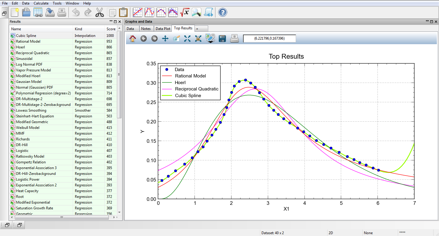
Spline functions and parametric spline curves have already become essential tools in data fitting and complex geometry representation for several reasons: being polynomial, they can be evaluated quickly; being piecewise polynomial, they are very flexible. The flexibility of splines provides best fitting results in most cases when the underlying math of the data is unknown. You can become convinced of this trying to find best approximation of your data using CurveExpert. By selecting Tools->CurveFinder… you can search for best data fit. After that call spline interpolation by selecting Calculate->Polynomial Spline… and enter spline degree. In most cases spline interpolation is the best fit.

Spline interpolation is a form of interpolation where the interpolant is a special type of piecewise polynomial called a spline. Being very useful in data fitting, interpolating splines are not the only possible way of restoring implicit relation with splines. On the contrary — interpolating splines are just a particular case of a more general superset of spline functions called smoothing splines.

If there is no restriction that fitting curve must pass exactly through data points, we can use different approach in fitting data with splines, reducing a total amount of piecewise polynomials that represent spline curve, and thus — eliminating side effects like overfitting, unpredictable behaviour on extrapolation (like that one at the picture above) etc. Application of smoothing splines produce smoother (than in the case of interpolating splines) but still flexible curves giving us some extra control over the curve shape and behaviour.

SciPy’s fitpack2 module (which is a part of the interpolate module) provides a pretty useful set of classes that represent univariate and bivariate splines. It is based on the collection of Fortran routines DIERCKX and provides object-oriented wrapping to this low-level functionality.

Further I will speak about univariate splines, but I’m pretty sure that similar operations can be scaled up to bivariate splines.

To construct univariate spline object you can instantiate one of the three classes:

• UnivariateSpline,
• InterpolatedUnivariateSpline,
• LSQUnivariateSpline,

passing them datapoints, spline degree, knot vector (for LSQUnivariateSpline) and optional additional parameters like weight vector, smoothing factor and boundary of the approximation interval.

Being a superclass for others, UnivariateSpline has the ability to be constructed in the alternative way: by passing it a tuple of knot vector t, B-spline coefficients c and spline degree k. This is implemented via _from_tck() classmethod. I find it pretty useful in creating new spline instances from others and in constructing parametric spline curves.

Here we need to understand the difference between spline functions (which we can construct in SciPy by instantiating any of the mentioned fitpack2 classes) and parametric spline curves.

Spline function \(y=f(x)\) maps a real number \(x\) to a real number \(y\); its knot vector is defined in the same space as \(x\) (in other words, represents position of knots along \(x\)-axis), while knots have to be in the ascending order. This can lead to some problems, like representing vertical lines.

Spline curve \(f(t)=(x(t),y(t))\) is represented by two distinct spline functions that use the same knot vector in its own parameter space \(t\). So we can say that parametric spline curve is a combination of two (or more in the space of higher degree) spline functions. That gives us the ability to represent much more complex shapes.

Another important property of parametric spline curves is the ability to define them through their control polygons, or in other words, control points.

Parametric spline curves and surfaces nowadays are widely used in modern CAD and computer graphics systems, allowing representation of complex shapes. Both creation and modification of spline curves are generally related to the processes of defining and moving their control points. This gives the designer control over the spline shape in a natural and explicit way as the curve is attracted to its control points.

The same approach can be applied to find accurate data fitting with parametric spline curves by adjusting positions of control points manually (or defining some algorithm to automate this process, which will be the topic of the future posts). The purpose of this topic is to show you that such approach can produce the best fitting results, while preserving low length of the spline’s knot vector and keeping it smooth.

So let’s take a look at the process of constructing parametric spline curves with SciPy:

1. Import numpy, matplotlib and SciPy’s interpolate module:

   import numpy as np
   import matplotlib.pyplot as plt
   import scipy.interpolate as si 
   

2. Define some control points and set some variables:

   x = [6, -2, 4, 6, 8, 14, 6]
   y = [-3, 2, 5, 0, 5, 2, -3]
   
   xmin, xmax = min(x), max(x) 
   ymin, ymax = min(y), max(y)
   
   n = len(x)
   plotpoints = 100
   

3. Next, set spline degree and find knot vector:

   k = 3
   knotspace = range(n)
   knots = si.InterpolatedUnivariateSpline(knotspace, knotspace, k=k).get_knots()
   knots_full = np.concatenate(([knots[0]]*k, knots, [knots[-1]]*k))
   

   Actually we could define knot vector manually, but to get smooth spline and avoid some difficulties we’ve just extracted knots from the instance of the InterpolatedUnivariateSpline class.

4. Now we need to construct tuples of knots, coefficients, and spline degree:

   tckX = knots_full, x, k
   tckY = knots_full, y, k
   

   Here we pass coordinates of control points as spline coefficients. This provides independence of control points on knots for the parametric spline curve and assures its free-form property.

5. Finally, construct two spline functions out of these tuples using _from_tck() classmethod:

   splineX = si.UnivariateSpline._from_tck(tckX)
   splineY = si.UnivariateSpline._from_tck(tckY)
   

6. Now we can evaluate our parametric spline curve for the set of parameter values tP :

   tP = np.linspace(knotspace[0], knotspace[-1], plotpoints)
   xP = splineX(tP)
   yP = splineY(tP)
   

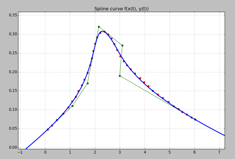
So let’s take a look at the spline functions and the parametric spline curve they represent:

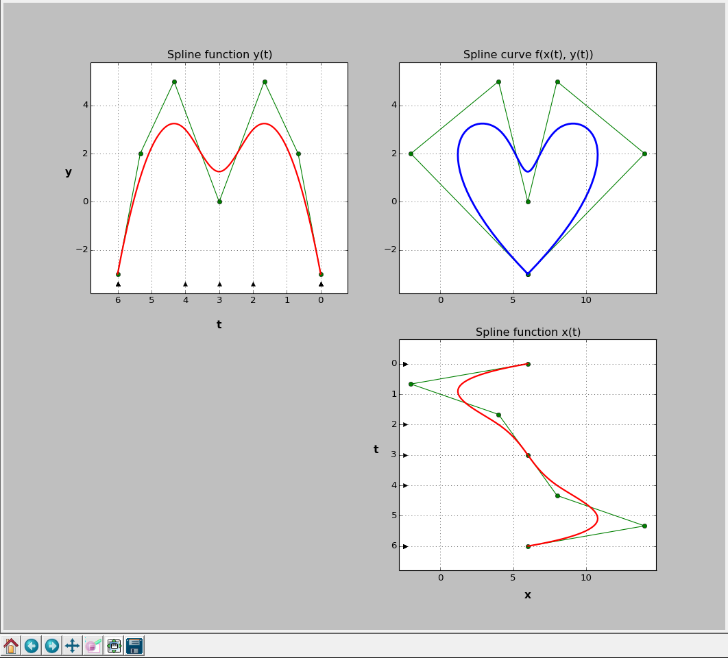
Here you can find a full example of building parametric spline curves with SciPy

Black triangles along parameter axes represent knots. Green polygons are actually the control polygons of the parametric spline curve and the support spline functions.

While control polygons of parametric spline curves are defined by coordinates in x and y, they do not depend on knot values. On other hand, control polygons of spline functions do depend on the coordinates of knots. To be more specific, coordinates of spline functions’ control points are points \((cp_i,x_i)\) and \((cp_i,y_i)\) where

are coordinates of control points along the parameter axis \(t\), while \(t_i\) are knots and \(k\) is a degree of the spline function.

So, to evaluate control points we can define a simple function:

def getControlPoints(knots, k):
    n = len(knots) - 1 - k
    cx = np.zeros(n)
    for i in range(n):
        tsum = 0
        for j in range(1, k+1):
            tsum += knots[i+j]
        cx[i] = float(tsum)/k
    return cx

cp = getControlPoints(knots_full, k)

Alteration of spline’s shape by editing its control points is quite challenging for spline functions. Assume we decided to edit control points of some spline function. Moving points along vertical axis is not a problem, as knot vector is independent on spline coefficients. But if we try to move points along the parameter axis we face the need to rebuild knot vector. To do that we hopefully would like to solve a linear equation system:

complemented with some boundary conditions. We can even get the solution, but there is no guarantee that knots will be in the ascending order. Moreover, if we add boundary conditions, based on the knowledge that the first and the last k+1 knots must be equal, we get overdetermined system.

That’s why instead of spline functions we would like to use easy-editable parametric spline curves, as their control points are independent on the knot vectors.

Now let’s compare the proposed approach of using parametric spline curves against three types of univariate smoothing spline functions provided by SciPy’s fitpack2 module in approximating some real engineering data.

2. Case Study

Assume we have some data and we need to find smooth spline approximation with the knot vector of minimal length:

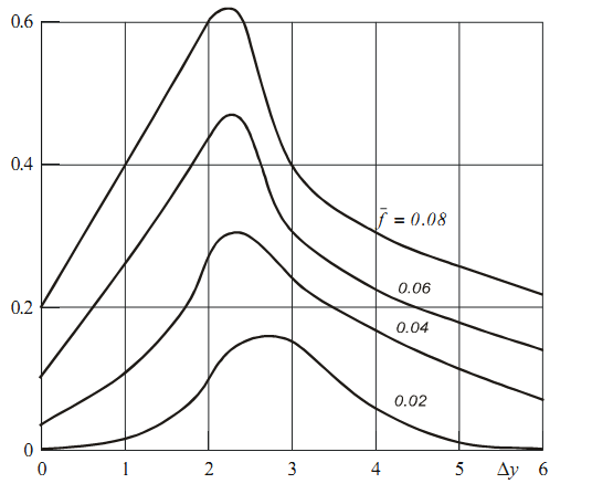
If you are interested in the nature of the data on the graph: these are dependencies of additional aerodynamic lift coefficient on the wing aspect ratio. Separate curves stand for wing profiles with different curvature. Let’s take the second curve from the bottom (one with the value of curvature ratio \(\bar{f} = 0.04\)) and try to find best possible approximation with splines.

But first of all we need to extract data points from the scanned image. I used Gsys application for this purpose but there are many alternatives. By picking points from the graph with Gsys we obtain vectors x and y that contain coordinates of data points:

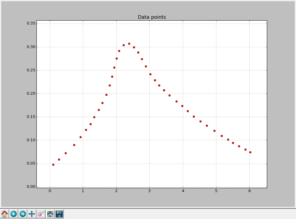
Here you can find data points picked from the graph with Gsys

Before we start building splines, it’s better to define the vector of weights w in order to force our further approximations to pass close to the end points of the original data:

wend = 3
w = [wend] + [1]*(num_points-2) + [wend]

Here num_points is the number of data points. In this way we obtain weight vector in the form: [3, 1, 1, ... 1, 1, 3]. If we pass this weight vector to any of the spline objects, resulting splines will be forced to stick to the first and the last data points since they have much higher weight.

First let’s find least squares spline approximation with SciPy.

2.1 Least Squares Spline Approximation

As LSQUnivariateSpline class requires knot vector on the call, we need to construct one somehow. At first let’s try to go with the uniform knot vector:

1. Construct uniform knot vector:

   knot_offset = (xmax - xmin)/(nknot + 1)
   knots = np.linspace(knot_offset, xmax-knot_offset, nknot)
   

   nknot - is the number of knots in the reduced knot vector (one without k repeating values at the endings). I put nknot = 3.

2. Instantiate LSQUnivariateSpline class using coordinates of the data points, the knot vector and the weight vector:

   lsqspline = si.LSQUnivariateSpline(x, y, knots, k=k, w=w)
   

3. Get full-length knot vector, spline coefficients and coordinates of control points along the x-axis:

   knots = lsqspline.get_knots()
   knots_full = np.concatenate(([knots[0]]*k, knots, [knots[-1]]*k))
   coeffs_y = lsqspline.get_coeffs()
   coeffs_x = getControlPoints(knots_full, k)
   

4. Evaluate spline points and plot the result:

   xP = np.linspace(x[0], x[-1], nsample)
   yP = lsqspline(xP)
   

   Here nsample - is the number of sample points for the spline to be evaluated at. It should be much more than the amount of data points. I put nsample = 100.

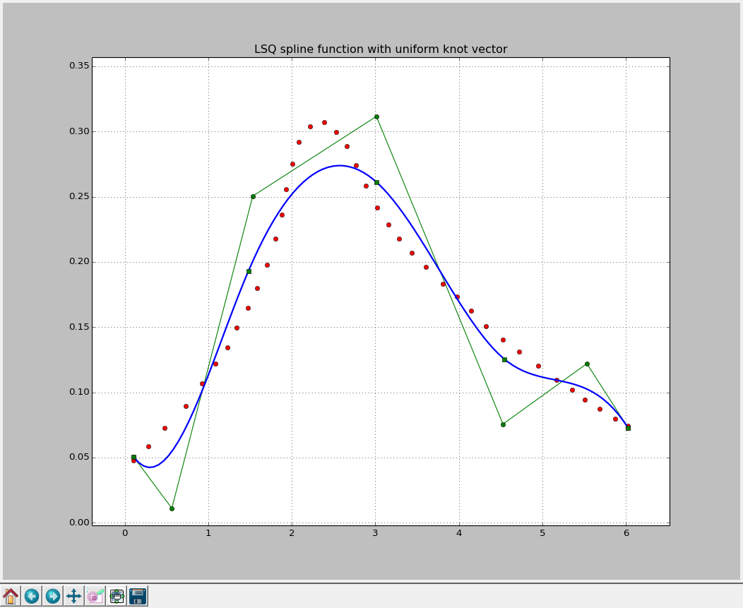
Well, as you can see this is definitely not the approximation we are looking for. And please believe me, varying the length of the knot-vector will not make it better. The problem is in the uniformity of the knot vector.

So, the next step is to try doing the same but with the non-uniform knot vector. You can achieve this either by inventing some efficient algorithm to construct best-fitting non-uniform knot vector iteratively (which is, actually a non-trivial task) or by selecting values of interior knots manually. For the sake of complexity reduction of the current example I’ve chosen the second way and it took me about 30 minutes to find good knot values:

knots = [1.2, 1.85, 2.0, 2.8, 3.5]

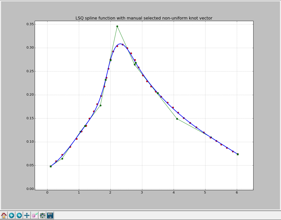
As you can see, this is a completely different story and I was pretty happy to find such a good fitting by adjusting values of the knot vector manually! I had to increase the length of the knot vector, which decreased smoothness of the spline a bit but allowed me to tune its behaviour on each section.

Unfortunately, if we evaluate our non-uniform spline to a wider boundaries, we can see that its extrapolating behavior, frankly speaking, is far from being satisfying:

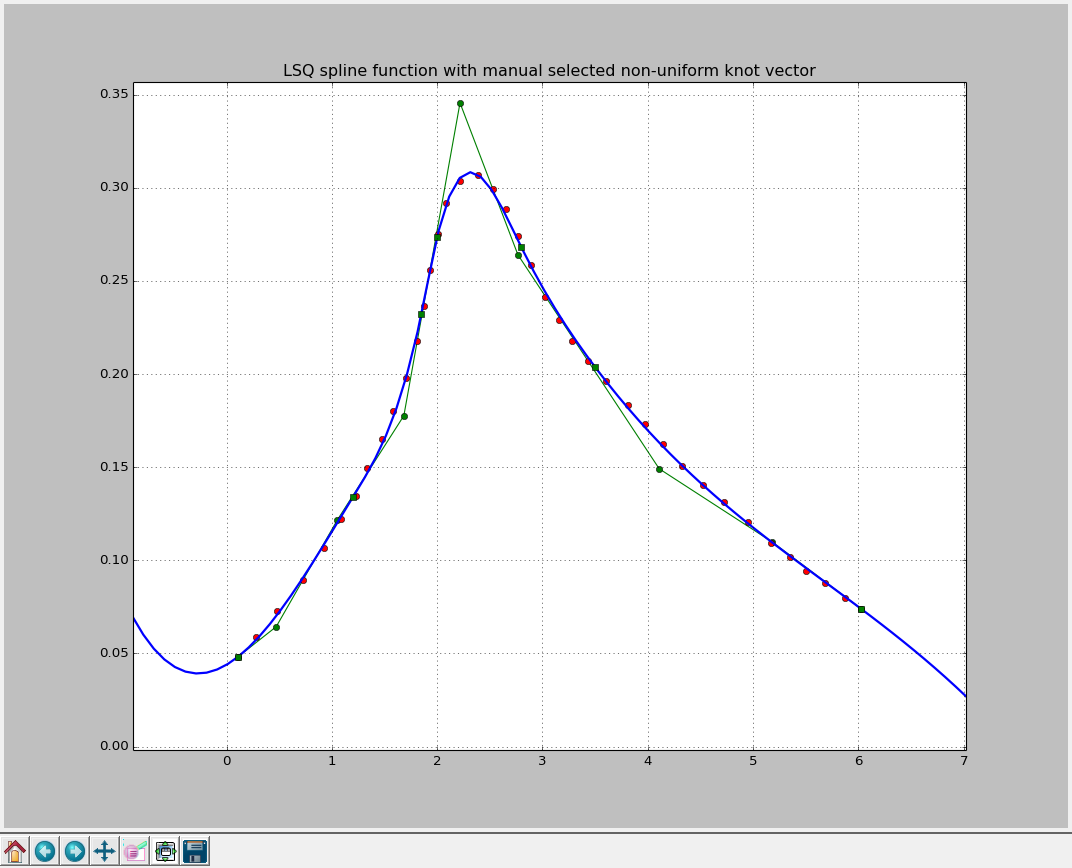
So, if we seek not only for the interpolation but extrapolation as well, we need to play with knot vector values for some more time or choose a different approach.

2.2 Smoothing Spline Approximation

We can avoid the necessity of defining knot vector by using UnivariateSpline class and passing it the smoothing factor s on the call. Let’s try to fit our data with different values of smoothing factor.

s = 0.1

spline = si.UnivariateSpline(x, y, k=k , s=0.1, w=w)
knots = spline.get_knots()
knots_full = np.concatenate(([knots[0]]*k, knots, [knots[-1]]*k))
coeffs_x = getControlPoints(knots_full, k)
coeffs_y = spline.get_coeffs()

xP = np.linspace(x[0], x[-1], nsample)
yP = spline(xP)

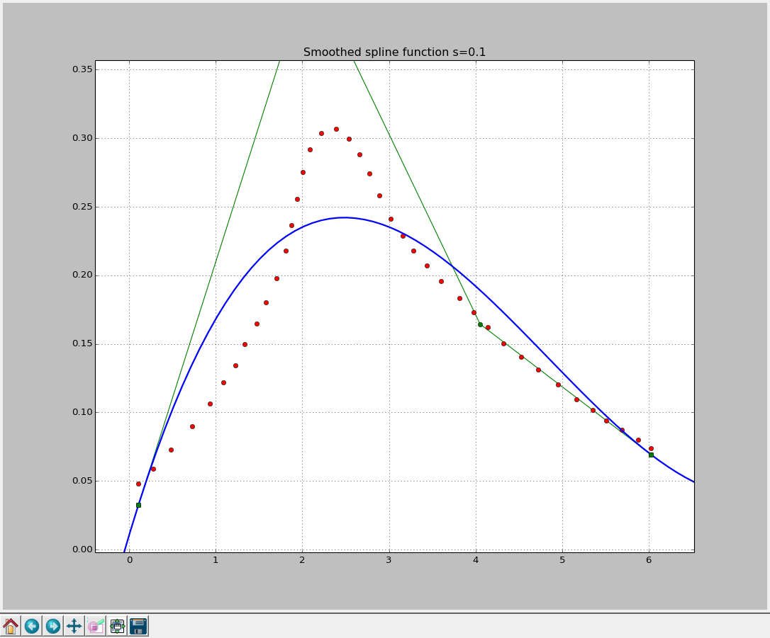
knots: [0.1062, 6.026]

Not even close…

s = 0.005

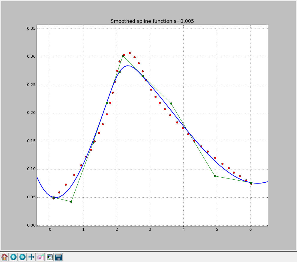
knots: [0.1062, 1.704, 2.086, 2.772, 6.026]

Better, closer, warmer!

A further decrease in the smoothing factor will lead to better results. But at the same time, knot vector length will increase. If we put s = 0 we get polynomial spline interpolation that we have already faced with:

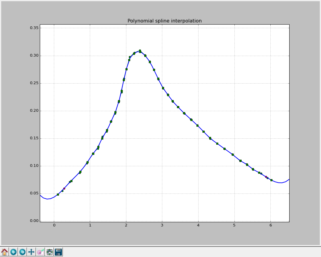
knots: [0.1062, 0.4779, 0.7301, 0.9292, 1.088, 1.227, 1.336, 1.473, 1.581, 1.704, 1.805, 1.877, 1.935, 2.007, 2.086, 2.216, 2.389, 2.534, 2.656, 2.772, 2.887, 3.024, 3.161, 3.284, 3.436, 3.602, 3.811, 3.977, 4.143, 4.323, 4.525, 4.72, 4.951, 5.167, 5.355, 5.507, 5.687, 6.026]

Because the inerpolating spline passes through each data point it’s not smooth, has data-long knot vector and behave badly on extrapolation. We can obtain the same result by calling InterpolatedUnivariateSpline class.

As we can see, curve fitting with smoothing spline functions can be a bit tricky, and the key to successful data fitting with spline functions is in finding custom non-uniform knot vector of minimal length.

So how can we benefit by applying parametric spline curves in data fitting?

2.3 Approximation with parametric spline curves

Let’s take the smooth spline function with s = 0.005 as the basis. First we will parameterize it and then we’ll edit its control points to find the best fitting.

To emphasize the independence of spline coefficients on the knot values I suggest you to norm the knot vector of the original spline function to some value. I’ve chosen the number of data points, but it can be any other number. Some usually simply take 1.

num_points = len(x)
num_knots = len(knots_full)
ka = (knots_full[-1] - knots_full[0])/(num_points)
knotsp = np.zeros(num_knots)
for i in range(num_knots):
    knotsp[i] = num_points - ((knots_full[-1] - knots_full[i]))/ka

Knot vector knotsp is defined in a new space, but relative position of knots hasn’t been changed, so the spline’s shape is preserved.

Now we need to repeat the same procedure that we started with to get parametric spline:

tckX = knotsp, coeffs_x, k
tckY = knotsp, coeffs_y, k
splineX = si.UnivariateSpline._from_tck(tckX)
splineY = si.UnivariateSpline._from_tck(tckY)

define control points’ coordinates along the parameter axis t:

coeffs_p = getControlPoints(knotsp, k)

and evaluate points of the curve:

tP = np.linspace(-3,  num_points+3, 100)
xP = splineX(tP)
yP = splineY(tP)

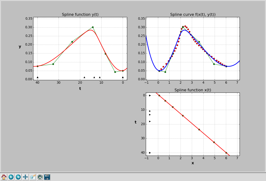
As we can see, spline function \(x(t)\) is a straight line what is obvious, as coefficients coeffs_p are just a scaled version of the original coeffs_x.

If I had this spline curve being represented in the window of some design software I just had to drag control points to the desired place until the curve will fit initial data points. To do this with matplotlib we need to use some additional framework for 2D graphics. But this will go straight out of the topic. Without that we just can manually select some new coordinates for control points. It’s pretty easy to do and took me about 10 minutes to get nice result. Of course it’s not what you would like to do every time you need to make an approximation but it satisfies our needs by now.

So, we have redefined control points, which are, actually coefficients of the support spline functions:

coeffs_x = [x[0], 1.1,   1.7,  2.16,  3.1,   3.0,   x[-1]]
coeffs_y = [y[0], 0.11,  0.17,  0.32,  0.27,  0.19,  y[-1]]

I put first and last coefficients to be equal to coordinates of first and last data points respectively. This ensures that resulting spline curve will pass through them.

Now we just need to rebuild spline curve with new coefficients:

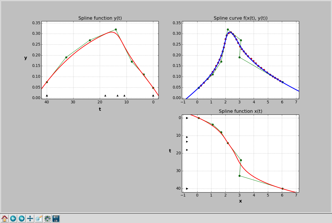
knots: [0.0, 10.79631069, 13.37747897, 18.0127707, 40.0]

This is obviously the best fitting result of all previous attempts. The curve is rather smooth, knot vector is short, and, what is also important, we have received good curve behaviour outside the data points.

However there is one significant challenge that we face while using parametric spline curves for data fitting. Since \(x\) and \(y\) depend on \(t\), there is no direct connection between \(x\) and \(y\) values. In other words, instead of common \(y = f(x)\) we obtain two dependencies in the form \(x = f(t)\) and \(y = f(t)\). This means we can’t evaluate \(y\) values directly as a function of \(x\), but have to find reversed dependency \(t = f(x)\) first. This increases complexity of spline points evaluation, which is the price for accuracy and flexibility.

Conclusions

SciPy provides ultimate tools for curve fitting with spline functions that in trained hands can be extremely helpful. Moreover, using this functionality we can easily construct parametric spline curves and by moving their control points achieve best approximation results. This can seem quite a rustic approach at first glance, but as we have noticed while trying different approaches, editing control polygon of parametric spline curve is much easier than finding proper knot vector for spline function.

Still, application of parametric spline curves for data fitting faces challenge of necessity to find reversed function \(t = f(x)\) to evaluate \(y\) as a function of \(x\). While this problem increases complexity of spline points evaluation, it has a solution, and I will describe how to find it with SciPy in the next article.

Curve Fitting with SplineCloud (update of Sep 2023)

The problem of finding the best fit to arbitrary data points has kept my mind strained for quite some time and has resulted in my endeavor to develop a general-purpose online spline fitting tool, which evolved into a spline management, and later into a general open knowledge management platform known as SplineCloud.

The SplineCloud interactive curve fitting tool allows to construct spline fit in one click. You can adjust the smoothing factor or select Least Squares or Interpolating splines. Manipulation of knot vectors and control points of splines is available in the Fine Tune mode. With this interactive curve fitting tool you can adjust the position of knots, add duplicate knots, move control points and change their weights. This approach of manual interaction have already proven to be helpful for data of complex shape.

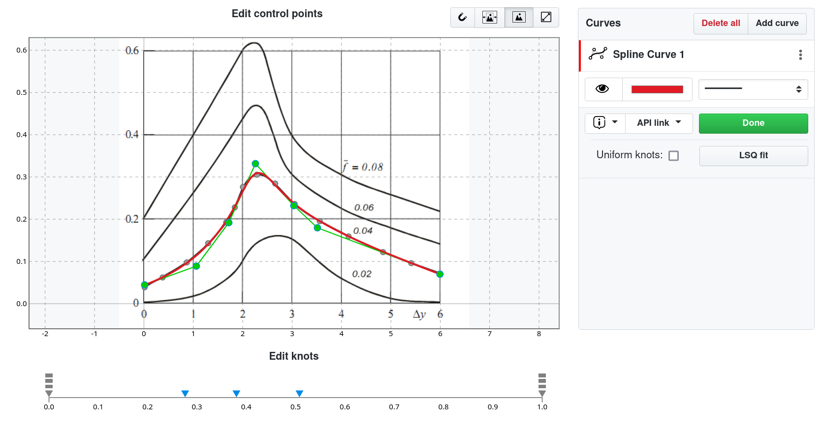
Most importantly, constructed curves can be pulled into your code by using SplineCloud client libraries for Python and MATLAB, and evaluated as regular functions!

Check out my article Online Curve Fitting with SplineCloud for more details.

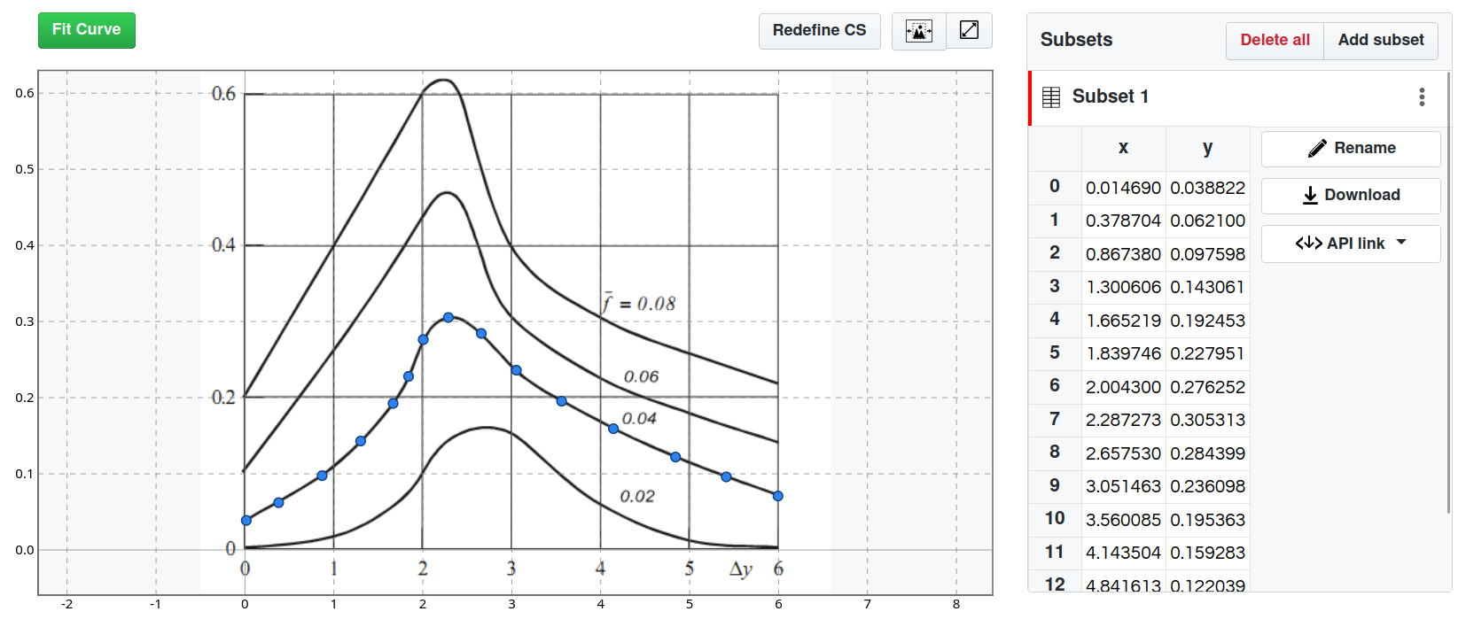
Plot Digitizing with SplineCloud (update of Sep 2023)

The solution for this problem has also found its place at SplineCloud. If your data is represented as a graph you can extract data points from it and go straight to finding the best fit. What is remarkable about this approach, is that you can display the original plot in the background, which allows you to find a more accurate fit by comparing the shapes of the original and fitting curves.

Examples

Example 1. Building Parametric Spline Curves with SciPy

Example 2. Data Points

Example 2. Spline Approximation with SciPy

References

[1] Michael S. Floater, “Splines and B-Splines”, INF-MAT5340-v2007, University of Oslo.

[2] Carl de Boor, “B(asic)-Spline Basics”, In Fundamental Developments in Computer-Aided Geometric Modeling, pages 27–49. Academic Press, London, UK, 1993.

[3] Ching-Kuang Shene, Introduction to Computing with Geometry Notes, Department of Computer Science, Michigan Technological University.

[4] SciPy Reference: scipy.interpolate